An introduction to Artificial Neural Network Optimizers (Part 2)

Introduction

In the first part of this two-part series on Neural Network Optimization, we discussed what Artificial Neural Networks are and how optimization algorithms are used to increase their performance. In addition, we had a look at the three most commonly used optimization algorithms: Gradient Descent (including variants such as Stochastic Gradient Descent and Mini-batch Gradient Descent), Momentum, and Nesterov Accelerated Gradient.

However, due to the widespread popularity of Artificial Neural Networks and the demand for increasingly more performant algorithms, researchers have come up with more novel approaches to optimize neural network parameters. These algorithms — including AdaGrad, RMSProps, Adam, and AdaDelta — will be the topic of the second part on this series on Neural Network Optimization.

AdaGrad

In the previous article we learned that classical optimization algorithms like Gradient Descent, Momentum, and Nesterov Accelerated Gradient determine the size and the direction of the neural network’s parameters update by looking at the slope of the error function — which is represented by a non-convex optimization surface. In addition, these algorithms take the tunable hyperparameter

(the learning rate) as an input — allowing one to influence the update size and thereby the time until the algorithm reaches convergence.

One of the problems with this methodology is that the learning rate remains constant throughout the optimization process. However — ideally –, we would like to increase the learning rate when the algorithm comes across features that are infrequent in the dataset and to decrease the learning when the algorithm comes across features that are frequent in the dataset.

This brings us to the second problem: apart from the learning rate being constant in time, it is also constant for each individual parameter. Instead, we would rather have an algorithm that can differentiate between parameters by making the update either smaller or larger for individual parameters by looking at their importance.

This is exactly what AdaGrad does: instead of having a learning rate which is constant throughout time and is constant for each individual parameter, AdaGrad updates the learning rates for all individual parameters after every parameter update step. Therefore, instead of representing the learning rate by a single scalar value (as was the case with previously discussed algorithms), AdaGrad uses a vectorized learning rate in which every parameter is assigned to an individual learning rate. This is mathematically shown in Equation 1 and Equation 2.

With representing a diagonal matrix which contains the sum of all the squared gradients related to up until update step and representing a smoothing term to avoid division by zero.

In vectorized form, the update step becomes the following:

The advantages of using the AdaGrad optimization algorithm are manifold. First, it does not require the user to tune the learning rate manually — as this is all handled by the algorithm itself. In addition, due to the learning rate being calculated and changed for each parameter during each iteration, the algorithm is able to learn on more versatile datasets — including very small and very sparse datasets.

Naturally, this is a disadvantage as well since it is computationally expensive to recalculate the learning rate during each iteration and for every parameter instead of selecting a constant. In addition, the way that the learning rates are being calculated (Equation 2) causes them to shrink during each iteration — ultimately resulting in all learning rates becoming equaling zero which causes learning to halt.

AdaDelta

The AdaDelta optimization algorithm is an improvement to AdaDelta in that it aims to circumvent the problem with shrinking learning rates by limiting the number of squared gradients that are taken into account when calculating the learning rates.

Instead of taking into account all the squared gradients related to up until update step (Equation 2), the AdaDelta optimization algorithm redefines the calculation of the learning rates as follows:

With representing a decaying average of al the squared gradients related to up until update step, which can be defined recursively as follows:

In vectorized form, the update step of the AdaDelta optimization algorithm can be formulated mathematically as follows:

The advantages of the AdaDelta optimization algorithm are straightforward. Instead of having shrinking learning rates — as was the case during AdaGrad optimization –, the AdaDelta optimization algorithm does not experience this behavior and is capable to continue learning indefinitely. However, the algorithm is still computationally expensive due to having to recalculate the learning rate during each iteration and for every parameter.

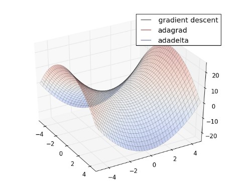
Figure 1: Comparison for time until convergence between regular gradient descent (green), AdaGrad (red) and AdaDelta (blue)

RMSprop

First suggested by Geoffrey Hinton during a lecture on Neural Networks for machine learning, RMSprop is an optimization algorithm that is in fact identical to the AdaDelta optimization algorithm. The sole difference between the two algorithms lies in the fact G. Hinton suggested to use a fixed value for and as default hyperparameter values during the optimization process.

Mathematically, this changes the parameter update step as follows:

Evidently, the advantages of the RMSprop optimization algorithm are similar to those of the AdaDelta optimization algorithm: it does not experience shrinking learning rates and is therefore capable of learning indefinitely. However — as is the case with AdaDelta and AdaGrad — the RMSprop algorithm is still computationally expensive due to having to recalculate the learning rate during each iteration and for every parameter.

Adam

At last, the Adam optimization algorithm — short for Adaptive Moment Estimation — has the same working principles as RMSprop and AdaDelta apart from the fact that — in addition to using the squared gradients — it also uses the regular gradients for calculating the learning rates.

Like Equation 4, the decaying averages of both the regular gradients and the squared gradients can be calculated as follows:

Using these values, the update step of the Adam optimizer can be denoted as follows:

Like the previously discussed algorithms, Adam optimizer does not experience shrinking learning rates and is therefore capable of learning indefinitely. In addition, Adam optimization is also considered to be one of the fastest algorithms to reach convergence — therefore making it the default optimizer choice for most neural network optimization that is being done today — with the proposed default parameters being

Comparing different Optimizers

Choosing which optimizer to use is highly dependent on the problem and the dataset at hand. Figure 1 and Figure 2 show the time-lapse of two optimization problems using different optimization algorithms. In general, adaptive learning rate algorithms such as AdaGrad, RMSprop, AdaDelta, and Adam outperform classical optimization algorithms such as gradient descent (Figure 1) and Stochastic Gradient Descent (Figure 2). However, setups in which Stochastic Gradient Descent are used in combination with momentum strategies are also heavily used within academic research– mostly due to their practical ease of implementation.

Figure 2: Comparison for time until convergence between Stochastic gradient descent (red), AdaGrad (blue), RMSprop (green), AdaDelta (purple), and Adam (yellow)

Conclusion

In this final article of the series on Artificial Neural Network Optimizers, we had a look at a selection of more novel optimization algorithms. More specifically, we discussed several optimizers which have adopted the practices of adaptive learning in order to drastically decrease the time to reach convergence — thereby distinguishing themselves from more classical optimization algorithms such as Gradient Descent variants and Momentum methodologies.